2017-06-10
課程教材作者群
課程教材作者群
名人堂:
Johnson Hsieh 
Wush Wu 
Rafe C. H. Liu 
GU Chen 
LIYUN 
大家好!我是 Lin!
33% Data Analyst + 33% Backpackers + 33% Coffee Hunter
些許經歷:
Data Analyst Intern at Whoscall 
Data Analyst Intern at DSP 
2016 Asia Open Data Hackathon Top1 
健保資料庫研究
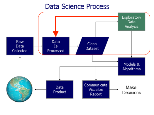
Data ETL 課程大綱
Agenda
- Data Input / Output:學會 讀取不同種的資料格式與輸出。
- Data Manipulation:學會 如何將資料操之在手。
- Data Aggregation: 學會 如何彙總出你有興趣的數字。
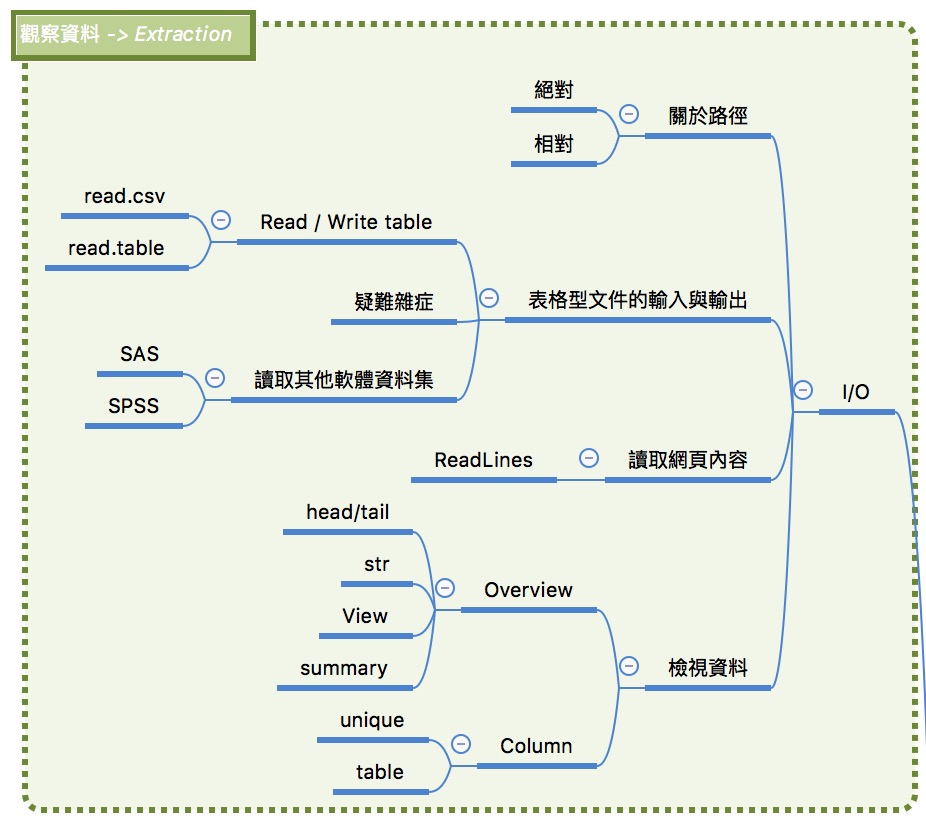
Data I/O:表格型文件的輸入與輸出
在讀檔案之前,先了解路徑的種類
路徑分為兩種:
- 絕對路徑:一般大家所認知的路徑長相。
- 相對路徑:從
working directory(工作目錄) 開始尋找
## 查看目前 Working directory 在哪個位置
getwd()
## 查看該工作目錄底下有什麼檔案
dir()
## 更改、設定工作目錄位置
# setwd('這邊放路徑')
輸入表格檔案(1/3)
- 下載範例資料
- 利用
read.csv讀取csv檔 (一種以逗點分隔欄位的資料格式) - 路徑必須指到下載的位置
############### 絕對路徑 ###############
# 請輸入完整的檔案路徑
transaction <- read.csv("/Users/sheng/Desktop/data/transaction.csv") #如果你是mac
transaction <- read.csv("C:\\Users\\transaction.csv") #如果你是windows
############### 相對路徑 ###############
# 設定我們檔案存放的路徑
setwd()
# 讀檔起手式
transaction <- read.csv("transaction.csv")
# 若讀入的是亂碼,猜猜看以下兩種編碼 utf-8 and big5
transaction <- read.csv("transaction.csv",fileEncoding = 'big5')
transaction <- read.csv("transaction.csv",fileEncoding = 'utf-8')
輸入表格檔案(2/3)
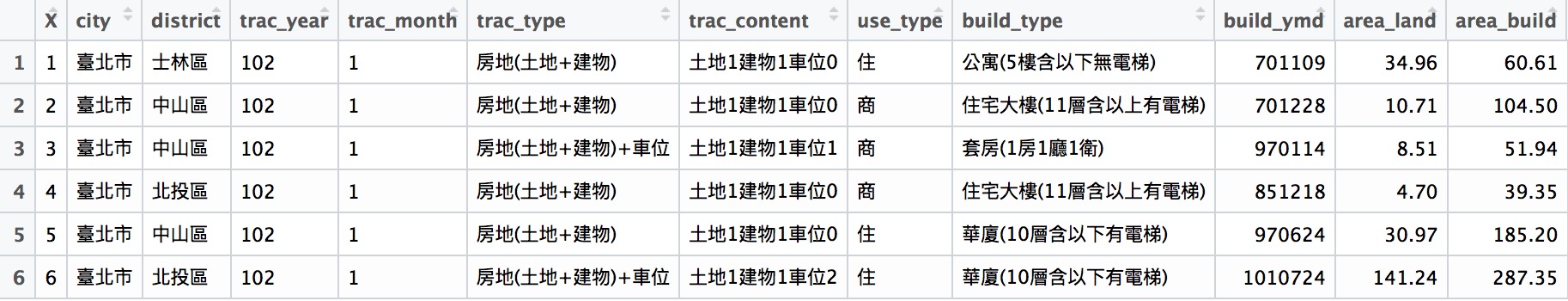
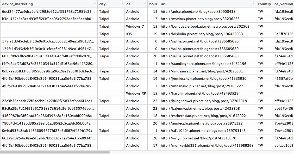
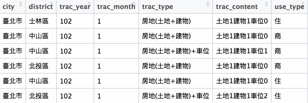
看看資料輸入後的結果有沒有問題:
transaction <- read.csv("data/transaction.csv")
head(transaction)
. . .
| 英文欄位名稱 | 中文欄位名稱 |
|---|---|
| city | 縣市 |
| district | 鄉鎮市區 |
| trac_year | 交易年份 |
| trac_month | 交易月份 |
| trac_type | 交易標的 |
| trac_content | 交易筆棟數 |
| use_type | 使用分區或編定 |
| 英文欄位名稱 | 中文欄位名稱 |
|---|---|
| build_type | 建物型態 |
| build_ymd | 建築完成年月 |
| area_land | 土地移轉總面積.平方公尺. |
| area_build | 建物移轉總面積.平方公尺. |
| area_park | 車位移轉總面積.平方公尺. |
| price_total | 總價.元. |
| price_unit | 單價.元.平方公尺. |
輸入表格檔案(3/3)
若是資料不如 csv 檔以 , 做分隔呢?
read.table()可以解決上述的問題,透過?read.table()可以查看其中可以調整的參數。注意到sep =是指定要輸入的資料是用什麼符號做分隔,當 read.table() 的 sep = ','時,跟 read.csv() 是相同的。
transaction <- read.csv("data/transaction.csv")
transaction <- read.table("data/transaction.csv", sep = ',', header = T)
讀取JSON檔案 (1/4)
install.packages("jsonlite")
讀取JSON檔案 (2/4)
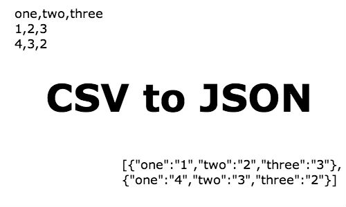
fromJSON: 將JSON轉換成 Factor, DataFrame, Matrix 等格式,?fromJSON查詢。toJSON:?toSON
json <-
'[
  {"Name" : "Mario", "Age" : 32, "Occupation" : "Plumber"},
  {"Name" : "Peach", "Age" : 21, "Occupation" : "Princess"}
]'
mydf <- fromJSON(json)
mydf
   Name Age Occupation
1 Mario  32    Plumber
2 Peach  21   Princess
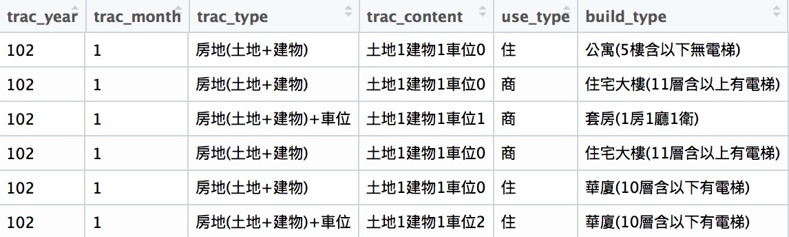
讀取JSON檔案 (3/4)
- 資料來源:2016-pixnet-hackathon-recommendation
- 資料長相:
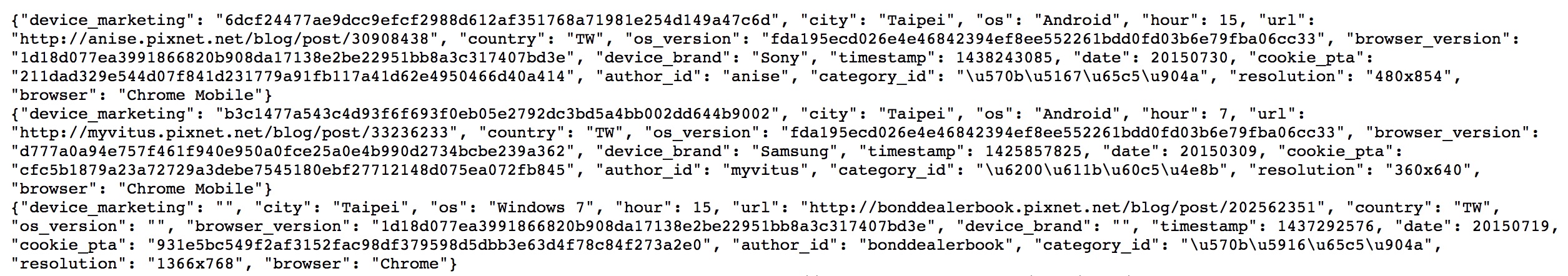
讀取JSON檔案 (4/4)
- 方法:使用
stream_in處理這種pseudo-JSON檔案
pixnet_json <- stream_in(url("https://raw.githubusercontent.com/pixnet/2016-pixnet-hackathon-recommendation/master/data/sample_training.json"))
head(pixnet_json)
輸出表格檔案
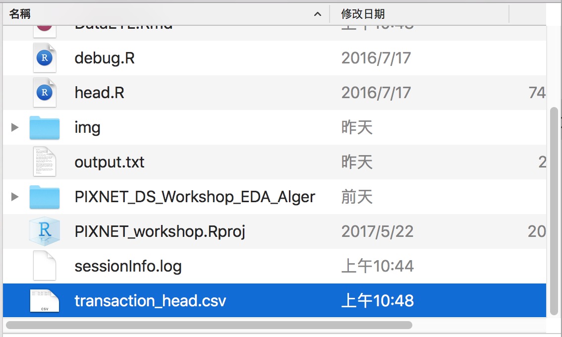
利用write.csv將data.frame格式的R物件另存成csv檔。為了效率,我們僅將 head(data) 6筆資料做輸出成 transaction_head.csv 即可。
write.csv(head(transaction), "transaction_head.csv", row.names=FALSE,quote=FALSE)
排解疑難 - 常見的讀取錯誤1
路徑錯誤
path <- "wrong_file_path"
dat <- read.csv(file = path)
Error in file(file, "rt") : 無法開啟連結
此外: Warning message:
  In file(file, "rt") : 無法開啟檔案 'wrong_file_path' :No such file or directory
- 絕對路徑 -> 確認檔案是否存在
- 相對路徑 -> 利用
getwd了解 R 當下的路徑位置
排解疑難 - 常見的讀取錯誤2
格式錯誤
path <- "data/transaction.csv"
dat <- read.csv(file = path, header = TRUE, sep = "1")
Error in read.table(file = file, header = header, sep = sep, quote = quote,  :
  more columns than column names
- 利用其他編輯器確認分隔符號
- 確認每列的資料的欄位是正確的
- 必要時,請用其他文件編輯器校正欲讀取的檔案
排解疑難 - 常見的讀取錯誤3
編碼錯誤
url <- "http://johnsonhsieh.github.io/dsp-introR/data/dsp-gift-2013-big5/%E8%B2%B7%E8%B3%A3st_A_10109_10109.csv"
dat <- read.csv(url)
Error in make.names(col.names, unique = TRUE) : 無效的多位元組字串於m
- 查詢檔案的編碼
- 常見的中文編碼有UTF-8和BIG-5
# 利用`fileEncoding`參數選擇檔案編碼 - big5 / utf8
dat2 <- read.csv(url, fileEncoding = "big5")
讀取其他軟體資料集
# install.packages("foreign") # 安裝R套件 foreign
library(foreign) # 載入套件
cars <- read.spss("data/Cars.sav", to.data.frame = TRUE)
milk <- read.dta("data/p004.dta")
# head(cars)
# head(milk)
讀取其他軟體資料集
- For SAS datasets, use the
sas7bdatpackage - airline: airline.sas7bdat
# install.packages("sas7bdat")
library(sas7bdat)
airline <- read.sas7bdat("data/airline.sas7bdat")
head(airline)
  YEAR   Y    W    R   L    K
1 1948 1.2 0.24 0.15 1.4 0.61
2 1949 1.4 0.26 0.22 1.4 0.56
3 1950 1.6 0.28 0.32 1.4 0.57
4 1951 1.9 0.30 0.39 1.5 0.56
5 1952 2.3 0.31 0.36 1.8 0.57
6 1953 2.7 0.32 0.36 1.9 0.71
Data I/O:讀取網頁內容(Lite)
逐行輸入與輸出
readLines,writeLines- 是讀取網頁原始碼的好工具
output <- file("output.txt")
writeLines(as.character(1:12), con = output)
input <- readLines(output)
input
[1] "1" "2" "3" "4" "5" "6" "7" "8" "9" "10" "11" "12"
練習
找出清心福全台北市南港店的地址
web_page <- readLines("http://www.319papago.idv.tw/lifeinfo/chingshin/chingshin-02.html")
# 如果你是windows, 這邊會遇到編碼問題,請加:
# web_page <- readLines("http://www.319papago.idv.tw/lifeinfo/chingshin/chingshin-02.html",encoding = 'UTF-8')
matches <- gregexpr("台北市南港區[\u4E00-\u9FA5|0-9]+", web_page)
tmp <- regmatches(web_page, matches)
unlist(tmp) # 把 list 轉成 vector
[1] "台北市南港區南港路3段20號" "台北市南港區南港路一段154號"
其中:
[\u4E00-\u9FA5]  :表示所有中文字符
|                 :表示 或
[0-9]              :含數字之字串
[a]+             :一或多個 a
此寫法為 正規表示法,後續將會在 字串處理 的主題中跟各位介紹。
小挑戰
- 找出清心福全台北市門市的電話號碼
- 提示:
"02-[0-9]+"
小挑戰
- 找出清心福全台北市門市的電話號碼
- 提示:
"02-[0-9]+"
參考解答:
web_page <- readLines("http://www.319papago.idv.tw/lifeinfo/chingshin/chingshin-02.html")
matches <- gregexpr("02-[0-9]+", web_page)
tmp <- regmatches(web_page, matches)
head(unlist(tmp))
[1] "02-28761717" "02-28311515" "02-28805757" "02-28829191" "02-28126988"
[6] "02-28835757"
Data I/O : 檢視資料
Recap 一下 Data I/O 我們學了什麼?
Data ETL 的第一步:輸入資料
- 設定資料路徑:
getwd()&setwd() - 輸入不同資料型態:
- 表格式:
read.csv()&read.table() - 網頁:
readLines() - 其他軟體:
read.sas7bdat()&read.spss() - 注意編碼、路徑設定、資料內容有沒有錯誤
- 表格式:
- 輸出資料:
write.csv()
輸入資料後下一步:檢視資料有無異常
輸入資料後,我們才準備正要開始 ETL 呢!
複習一下常用的資料檢視方式:
- 總覽
head(),tail():抓前五筆、後五筆資料str(),summary():檢視資料的結構、簡單敘述性統計View():自由瀏覽
- 單一欄位檢視
unique():檢視類別型欄位table():檢視類別型欄位
資料總覽
head(transaction)
  X   city district trac_year trac_month            trac_type
1 1 臺北市   士林區       102          1      房地(土地+建物)
2 2 臺北市   中山區       102          1      房地(土地+建物)
3 3 臺北市   中山區       102          1 房地(土地+建物)+車位
4 4 臺北市   北投區       102          1      房地(土地+建物)
     trac_content use_type                 build_type build_ymd area_land
1 土地1建物1車位0       住      公寓(5樓含以下無電梯)    701109      35.0
2 土地1建物1車位0       商 住宅大樓(11層含以上有電梯)    701228      10.7
3 土地1建物1車位1       商            套房(1房1廳1衛)    970114       8.5
4 土地1建物1車位0       商 住宅大樓(11層含以上有電梯)    851218       4.7
  area_build area_park price_total price_unit age
1         61       0.0     6380000     105263  32
2        104       0.0    12010000     114928  32
3         52       8.6    10080000     194070   5
4         39       0.0     4600000     116900  17
 [ reached getOption("max.print") -- omitted 2 rows ]
tail(transaction)
            X   city district trac_year trac_month            trac_type
153593 153593 新北市   三重區       102          4      房地(土地+建物)
153594 153594 新北市   三重區       102          6 房地(土地+建物)+車位
153595 153595 新北市   三重區       102          3      房地(土地+建物)
153596 153596 新北市   三重區       102          3      房地(土地+建物)
          trac_content use_type                 build_type build_ymd
153593 土地1建物1車位0       住 住宅大樓(11層含以上有電梯)   1021220
153594 土地1建物1車位1       住 住宅大樓(11層含以上有電梯)   1021220
153595 土地1建物1車位0       住 住宅大樓(11層含以上有電梯)   1021220
153596 土地1建物1車位0       住 住宅大樓(11層含以上有電梯)   1021220
       area_land area_build area_park price_total price_unit age
153593      10.6         81         0    11680000     143471   0
153594      12.5         97         0    15390000     158382   0
153595       8.3         64         0     9000000     140034   0
153596       8.3         64         0     9200000     143146   0
 [ reached getOption("max.print") -- omitted 2 rows ]
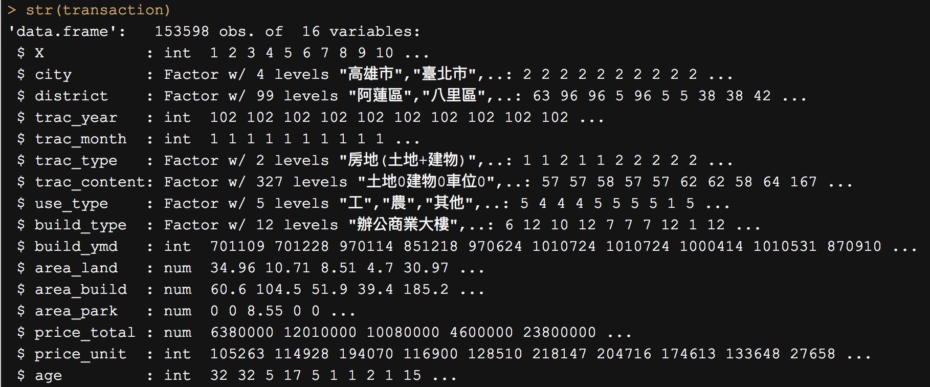
str() 會檢視資料中每個欄位的:型態(int, Factor, chr, …)以及值
str(transaction)
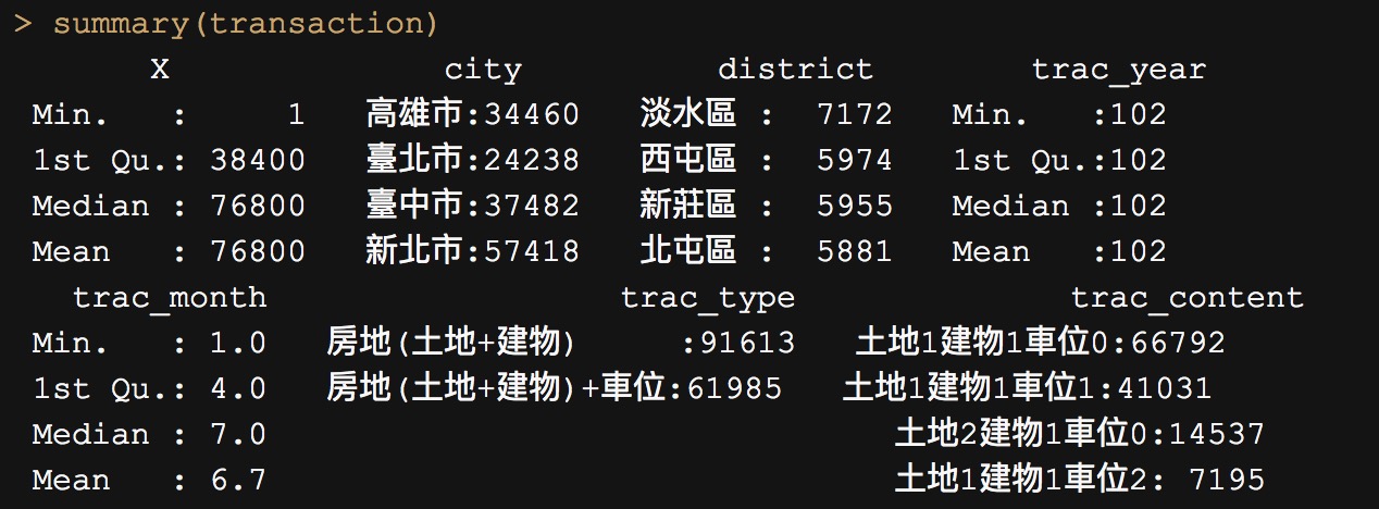
summary 會檢視資料中每個欄位敘述性統計(值的分佈)
summary(transaction)
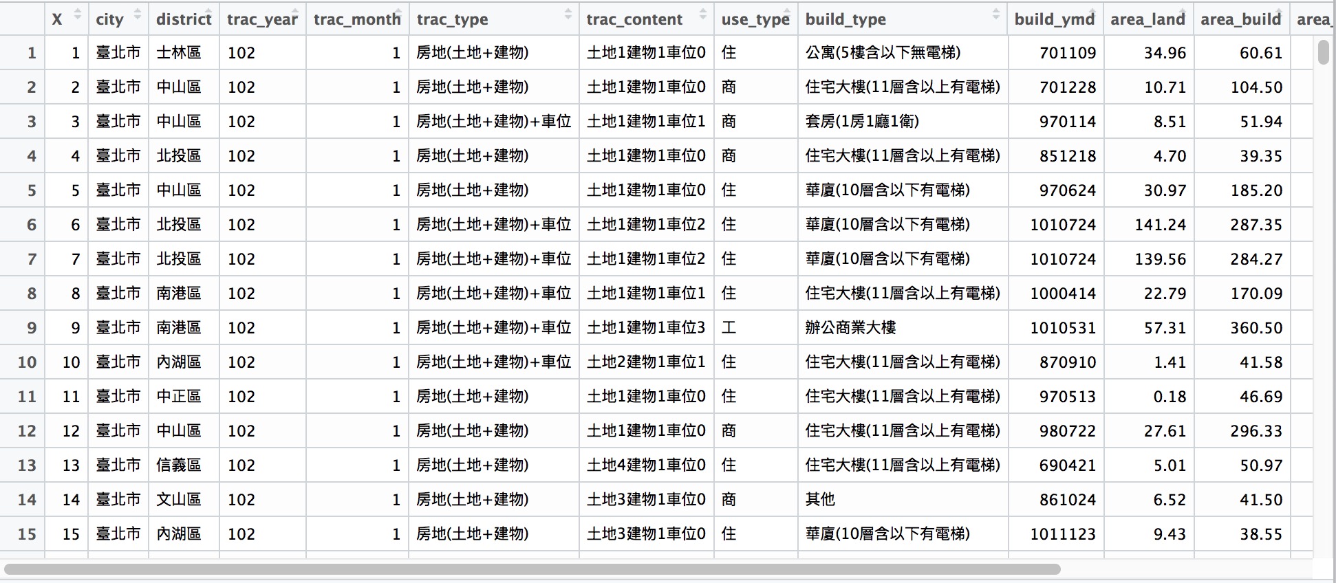
View()
View(transaction)
單一欄位檢視
table(transaction$city)
高雄市 臺北市 臺中市 新北市
 34460  24238  37482  57418
unique(transaction$district)
 [1] 士林區 中山區 北投區 南港區 內湖區 中正區 信義區 文山區 松山區 萬華區
[11] 大安區 大同區 北區   大里區 西屯區 太平區 南屯區 沙鹿區 東勢區 西區
[21] 豐原區 中區   北屯區 龍井區 后里區 烏日區 大雅區 南區   潭子區 大甲區
[31] 神岡區 東區   清水區 霧峰區 大肚區 梧棲區 新社區 外埔區 石岡區 左營區
[41] 苓雅區 鼓山區 小港區 三民區 鳳山區 楠梓區 新興區 前鎮區 路竹區 仁武區
[51] 林園區 前金區 岡山區 大寮區 鳥松區 大社區 鹽埕區 橋頭區 湖內區 阿蓮區
[61] 茄萣區 大樹區 梓官區 美濃區 旗津區 燕巢區 旗山區 永安區 六龜區 甲仙區
[71] 彌陀區 桃源區 中和區 三峽區 土城區
 [ reached getOption("max.print") -- omitted 24 entries ]
99 Levels: 阿蓮區 八里區 板橋區 北區 北投區 北屯區 大安區 ... 左營區
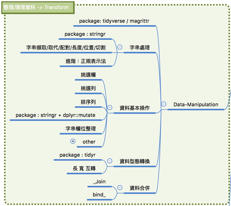
Data Manipulation
Data Manipulation: Pipe Line Coding Style
為什麼這邊要教 Pipeline Coding style ?
根據不具名調查指出,寫程式花了將近 80% 時間在思考如何命名物件名稱。
命名物件名稱是門藝術,當然我們也可以隨性命名:
## 假設我們現在要做這件事情
pixnet_good <- iris$Species
pixnet_good_again <- as.character(pixnet_good)
pixnet_good_again_again <- table(pixnet_good_again)
pixnet_good_again_again
pixnet_good_again
    setosa versicolor  virginica
        50         50         50
當然我們也可以這樣改寫,節省命名的時間:
table(as.character(iris$Species))
    setosa versicolor  virginica
        50         50         50
為什麼這邊要教 Pipeline Coding style ?
當整份 .r 檔都是這樣的寫法時,你會發現幾個問題:
- 解讀程式碼不直覺:我們習慣從外往內解讀
table -> as.character -> iris$... - 要改寫程式碼也較不容易
所以我們需要一個更直覺的工具幫助我們解決這些問題 …
2014 年最有影響的套件之一:magrittr
- 壓縮的程式碼不好讀
- 展開的程式碼會產生很多暫存變數
magrittr 套件聽到大家的聲音了!

- 運用
magrittr所開發的%>%進行 Pipeline coding style - 養成 Pipeline Style 的 coding 習慣,上述問題迎刃而解!
- Pipeline 快捷鍵(MAC):
command + shift + M - Pipeline 快捷鍵(WIN):
ctrl + shift + M
- Pipeline 快捷鍵(MAC):
基本算子 (%>%)
基本算子 (%>%)
- 想像一下程式的寫作與閱讀邏輯
%>%會將算子左邊的物件 (object) 傳到右邊的函數 (function) 中第一個 argument- . 點號適合用在欲傳入變數不是在傳入函數的第一個位置時使用
- use
x %>% f, rather thanf(x) - or use
x %>% f(y, z), rather thanf(x, y, z) - or
y %>% f(x, ., z), rather thanf(x, y, z) - 更多 Pipeline 請參考 Johnson Hsieh 的講義
# install.packages("magrittr")
library(magrittr)
x <- 1:10
x %>% mean # 由左而右順序操作
[1] 5.5
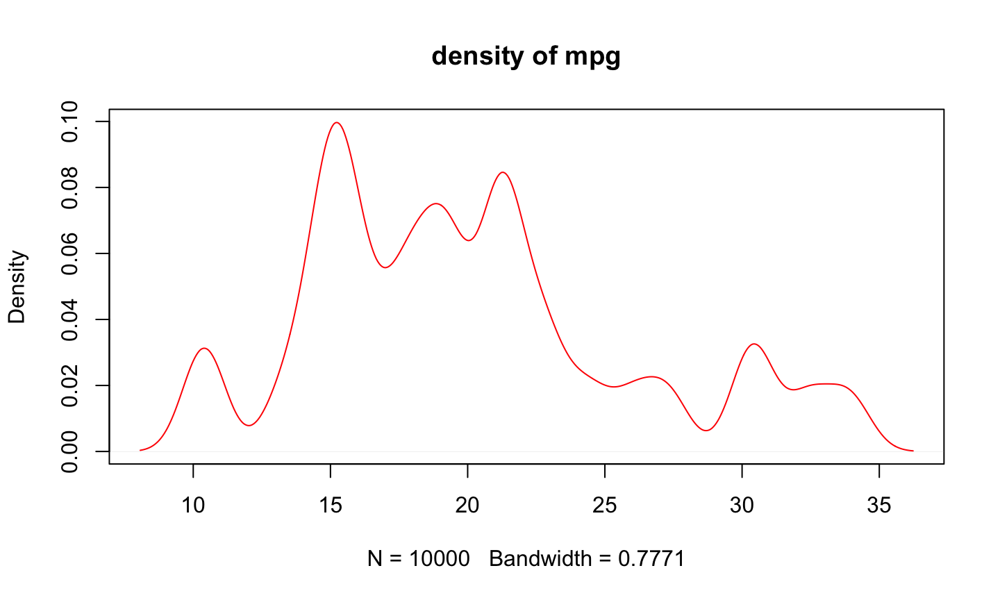
# 指令壓縮
plot(density(sample(mtcars$mpg, size=10000, replace=TRUE),
             kernel="gaussian"), col="red", main="density of mpg")

# Pipe Line
mtcars$mpg %>%
    sample(size=10000, replace=TRUE) %>%
    density(kernel="gaussian") %>%
    plot(col="red", main="density of mpg")
Data Manipulation : 字串資料處理
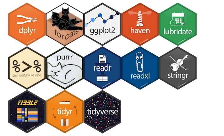
tidyverse 套件
stringr 是專門處理字串的一個知名套件,他與之後會介紹的強大套件 dplyr, tidyr, ggplot2 皆整合至 tidyverse 套件之中了。
tidyverse 套件安裝
我們先安裝 tidyverse 套件:
install.packages("tidyverse")
library(tidyverse)
library(stringr)
stringr 基本介紹
所有的 stringr 的 function 皆用 str_ 作為開頭(記得善用 Tab 鍵唷!)
我們用先前的 transaction 資料來練習一下字串處理吧!
以 transaction 的 build_ymd 建築年月日為例:
build_ymd <- transaction$build_ymd
build_ymd %>% head()
[1] 701109 701228 970114 851218 970624 1010724
stringr:str_length & str_sub 字串長度與字串擷取
- 目標:取出 build_ymd 的年、月、日
- 注意:字串的長度不同(6與7)
- 善用
?str_sub查詢 function 使用方法
year <- ifelse(str_length(build_ymd) == 6,
               str_sub(build_ymd, 1,2),
               build_ymd %>% str_sub(1,3)) # 這兩種寫法都可以
year_unique <- year %>% unique()
year_unique
 [1] "70"  "97"  "85"  "101" "100" "87"  "98"  "69"  "86"  "74"  "78"
[12] "99"  "67"  "90"  "71"  "75"  "73"  "68"  "94"  "62"  "10"  "92"
[23] "82"  "93"  "88"  "76"  "60"  "96"  "66"  "83"  "61"  "81"  "72"
[34] "95"  "65"  "89"  "79"  "64"  "63"  "57"  "80"  "84"  "58"  "91"
[45] "77"  "56"  "59"  "55"  "51"  "49"  "50"  "45"  "53"  "102" "15"
[56] "47"  "54"  "23"  "52"  "41"  "12"  "44"  "17"  "46"  "42"  "48"
[67] "38"  "27"  "24"  "103" "35"  "30"  "22"  "21"  "40"
 [ reached getOption("max.print") -- omitted 11 entries ]
若不寫 ifelse, 我們也可以:
- start = 1 : 從第一個開始
- end = -5 : 到倒數第五個
year_unique2 <- str_sub(build_ymd, 1,-5) %>% unique()
any(year_unique != year_unique2) # check 有沒有任何一個不一樣
[1] FALSE
stringr : str_detect 字串檢驗
- 目標:從 build_type 中判斷是否有電梯
- 善用
?str_detect查詢 function 使用方法
build_type_vector <- transaction$build_type
build_type_vector %>% str_detect('有電梯') %>% table
.
FALSE  TRUE
62508 91090
stringr : str_split 字串分割
- 目標:根據 fruit 中的 and 進行切割
- 善用
?str_split查詢 function 使用方法
fruits <- c(
  "apples and oranges and pears and bananas",
  "pineapples and mangos and guavas")
str_split(fruits, " and ")
[[1]]
[1] "apples"  "oranges" "pears"   "bananas"

[[2]]
[1] "pineapples" "mangos"     "guavas"
str_split(fruits, " and ", simplify = TRUE) # simplify = T > 回傳矩陣
     [,1]         [,2]      [,3]     [,4]
[1,] "apples"     "oranges" "pears"  "bananas"
[2,] "pineapples" "mangos"  "guavas" ""
stringr : str_replace 字串取代
- 目標:將 trac_type 中的
房地拿掉 - 善用
?str_replace查詢 function 使用方法
trac_type <- transaction$trac_type
trac_type %>% str_replace('房地','') %>% head
[1] "(土地+建物)"      "(土地+建物)"      "(土地+建物)+車位"
[4] "(土地+建物)"      "(土地+建物)"      "(土地+建物)+車位"
stringr : str_replace 字串取代
- 目標:將 trac_type 中的
(土地+建物)拿掉 - 善用
?str_replace查詢 function 使用方法
trac_type <- transaction$trac_type
trac_type %>% str_replace('(土地+建物)','') %>% head
[1] "房地(土地+建物)"      "房地(土地+建物)"      "房地(土地+建物)+車位"
[4] "房地(土地+建物)"      "房地(土地+建物)"      "房地(土地+建物)+車位"

正規表示法 Regular Expression
正規表示法是一種描述文字模式的語言,可以讓我們撰寫程式來自文字中比對、取代甚至是抽取各種資訊。
參考 Wush Wu 所撰寫的教材,開頭或結尾的簡單的例子:
^AA:表示以AA為開頭的規則AA$:表示以AA為結尾的規則
str_detect(c('AA1','A2','V3','AAA4','ACA21'),'^AA')
[1] TRUE FALSE FALSE TRUE FALSE
str_detect(c('AA1','A2','V3','AAA4','ACA21'),'1$')
[1] TRUE FALSE FALSE FALSE TRUE
(土地+建物)無法辨識的原因
stringr 中的 pattern參數預設使用正規表示法,剛剛我們所要比對的規則(土地+建物)中的(,+,)皆是正規表示法中的特殊符號,如果這些剛好是要比對的文字,那就要加上跳脫字元""。又剛好跳脫字元""也是R 的字串的跳脫字元,所以我們在輸入時,一個""就要輸入兩次。
trac_type %>% str_replace('\\(土地\\+建物\\)','') %>% head
[1] "房地" "房地" "房地+車位" "房地" "房地" "房地+車位"
Data Manipulation : 資料基本操作
2014 年最有影響的套件之一:dplyr
- 讓R 使用者可以用更有彈性的方式來處理資料
- 針對
data.frame做設計(名稱中的d) - 設計理念
- 導入資料整理最重要的動作(非常類似SQL)
- 快
- 支援異質資料源(
data.frame或資料庫中的表格)
學習dplyr的官方方式:vignette
vignette(all = TRUE, package = "dplyr")
vignette("introduction", package = "dplyr")
- 更詳細的dplyr介紹可以閱讀dplyr的小論文
- R 的開發者會針對一個主題撰寫小論文做介紹
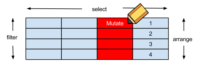
dplyr簡介
filter對列做篩選 (row)select對欄做篩選 (column)arrange排列mutate更改欄或新增欄- **
group_by+summarise分類
filter : 對列做篩選
filter : 對列做篩選
- 目標:取出 city 為 '臺北市'
library(dplyr) #載入套件
transaction %>%
  filter(city == '臺北市') %>% head
select : 對行做選取
select : 對行做選取
- 目標:取出
city,district,price_total欄位
transaction %>%
  select(city, district, price_total) %>%
  head()
    city district price_total
1 臺北市   士林區     6380000
2 臺北市   中山區    12010000
3 臺北市   中山區    10080000
4 臺北市   北投區     4600000
5 臺北市   中山區    23800000
6 臺北市   北投區    62000000
select : 對行做選取
也可以用負號-執行反向選取
transaction %>%
  select(-c(city, district, price_total))%>%
  head()
arrange : 資料排序
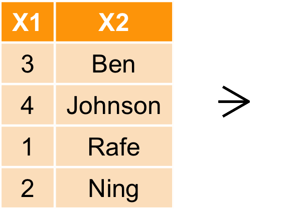
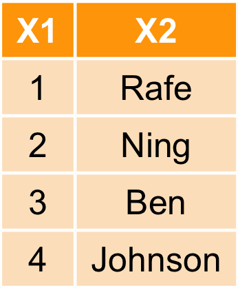
arrange : 資料排序
- 目標:按照總價格
price_total由小到大進行排序 - 注意:可以發現到 price_total 似乎有一些值不合理?(0)如何檢驗? -> ETL
transaction %>% arrange(price_total) %>% select(X,city, price_total) %>% head
      X   city price_total
1 53063 臺中市           0
2 59110 臺中市           0
3 74325 高雄市           0
4  4381 臺北市           1
5 50387 臺中市        1040
6 34755 臺中市        1380
arrange : 資料排序
- 排序預設是由小到大,加上
desc可使用遞增排列
transaction %>% arrange(desc(price_total)) %>%
  select(X,city, price_total) %>% head
      X   city price_total
1  2209 臺北市  8800000000
2 20777 臺北市  6680000000
3 49039 臺中市  4896000000
4 40626 臺中市  2800000000
5 49569 臺中市  2727360000
6 99765 新北市  2670000000
mutate : 新增欄位
mutate : 新增欄位
- 目標:根據
area_build,price_total自行計算單位坪價
transaction_new <- transaction %>%
  mutate(price_per_unit = price_total/area_build)
transaction_new %>% select(price_total, area_build, price_per_unit) %>% head
  price_total area_build price_per_unit
1     6380000         61         105263
2    12010000        104         114928
3    10080000         52         194070
4     4600000         39         116900
5    23800000        185         128510
6    62000000        287         215765
其他 dplyr 基本常用 function
- 移除重複資料:
distinct(transaction) - 隨機抽取資料:
sample_n(transaction, 5) - 抽取指定列:
slice(transaction, c(1,3,4,5)) - 更多請見dplyr Cheatsheet
Data Manipulation 小挑戰
- 目標:利用
build_type欄位挑出 有電梯 的資料 - 方法:
filter()+str_()
Data Manipulation 小挑戰參考解答
transaction %>%
  filter(build_type %>% str_detect('有電梯')) %>%
  head
小挑戰2
- 目標:請挑出 在台北市中山區與北投區的交易資料,並且新增
is_elevator是否有電梯的欄位,若有電梯則填入'TRUE',若無則填入'FALSE',並且以屋齡做遞增排序,僅保留city,district,age,price_unit等欄位。 - Tips : 多個條件配對可用
%in%。 ex:apple%in%c('apple', 'banana')
    city district age price_unit
1 臺北市   中山區   0     398552
2 臺北市   中山區   0     307621
3 臺北市   北投區   0     180279
4 臺北市   北投區   0     198974
5 臺北市   北投區   0     183904
6 臺北市   北投區   0     174448
transaction %>%
  filter(city == '臺北市', district %in% c('中山區','北投區')) %>%
  mutate(is_eleavator = str_detect(build_type, '有電梯')) %>%
  arrange(age) %>%
  select(city, district, age, price_unit) %>% head
Data Manipulation : 資料型態轉換
資料型態轉換 : Wide format <-> Long format
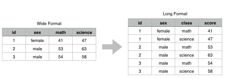
事實上 Long-format 的資料的格式不容易讓人類做比較。反而比較易於電腦讀取,人類在吸收資訊的時候更適合看 wide-format。
接著我們就來介紹如何做資料型態的轉換囉!long-format <-> wide-format
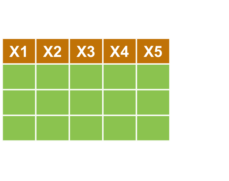
spread & gather : 長轉寬
接著我們來介紹 tidyr 中的 spread & gather 這兩個 Function:
?spread: key 擺放要展開的欄位,value 展開欄位後對應填入的值
library(tidyr) # 載入套件
long <- data.frame(id = c(1,1,2,2,3,3),
                   sex = c(rep('female',2),rep('male',4)),
                   class = rep(c('math','science'), length.out = 6),
                   score = c(41, 47, 53, 63, 54, 58))
wide <- long %>% spread(class, score)
wide
  id    sex math science
1  1 female   41      47
2  2   male   53      63
3  3   male   54      58
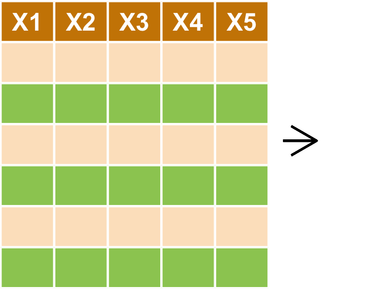
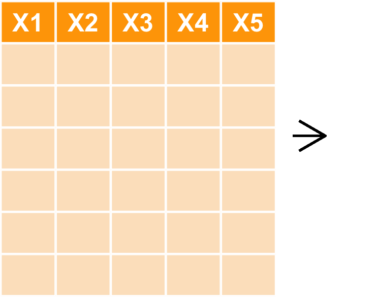
spread & gather : 寬轉長
?gather:- key、value : 皆放欄位名稱
-c(id, sex): 這兩個欄位不要轉換
wide %>%
  gather(key = 'class',value = 'score', -c(id,sex))
  id    sex   class score
1  1 female    math    41
2  2   male    math    53
3  3   male    math    54
4  1 female science    47
5  2   male science    63
6  3   male science    58
Data Manipulation : 資料合併
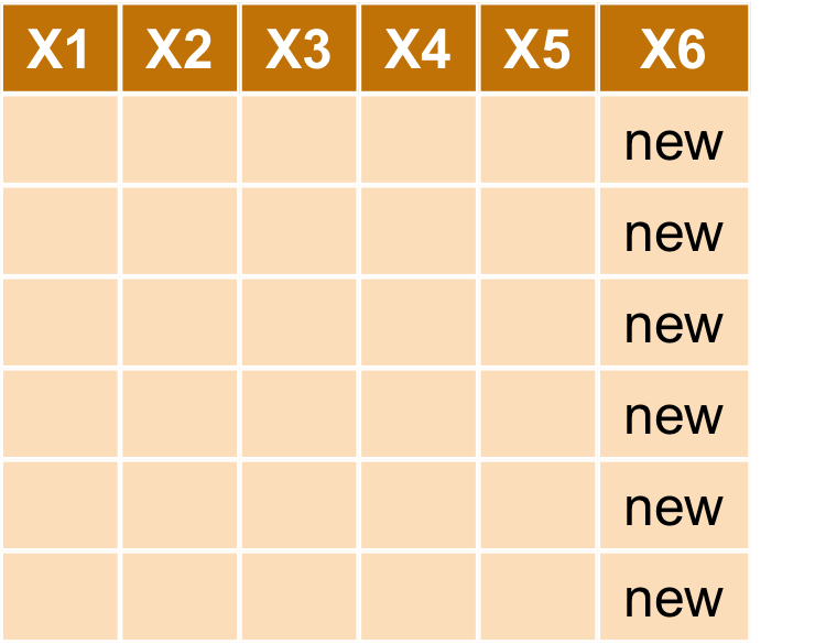
bind_ 資料表合併
- dplyr::
bind_rows()
- dplyr::
bond_cols

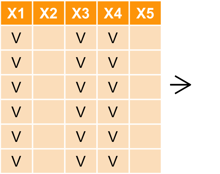
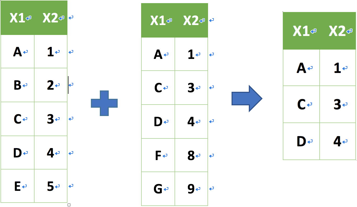
_join 資料表合併
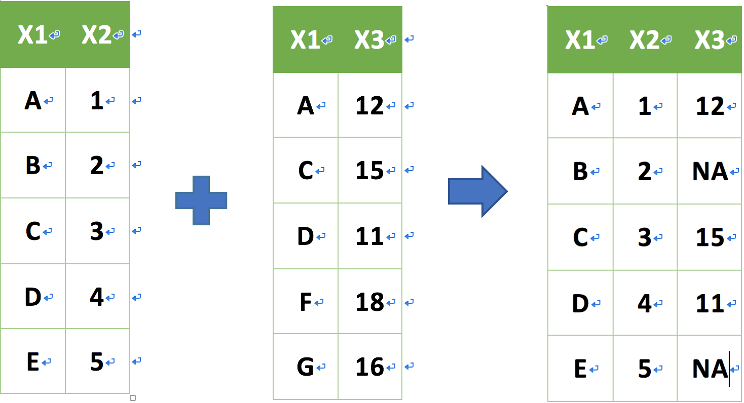
join family:left_join
left_join(a, b, by = "x1")
_join 資料表合併
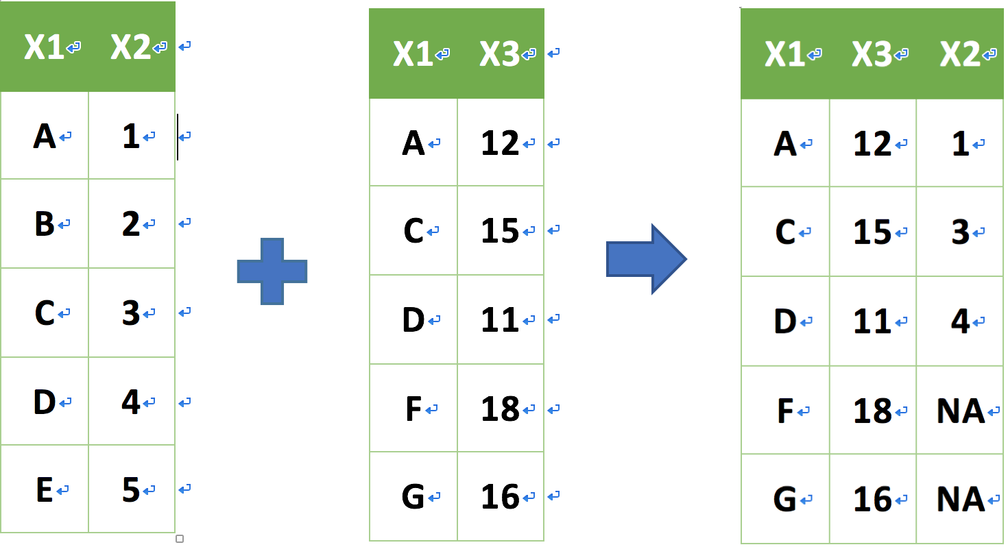
join family:right_join
right_join(a, b, by = "x1")
_join 資料表合併
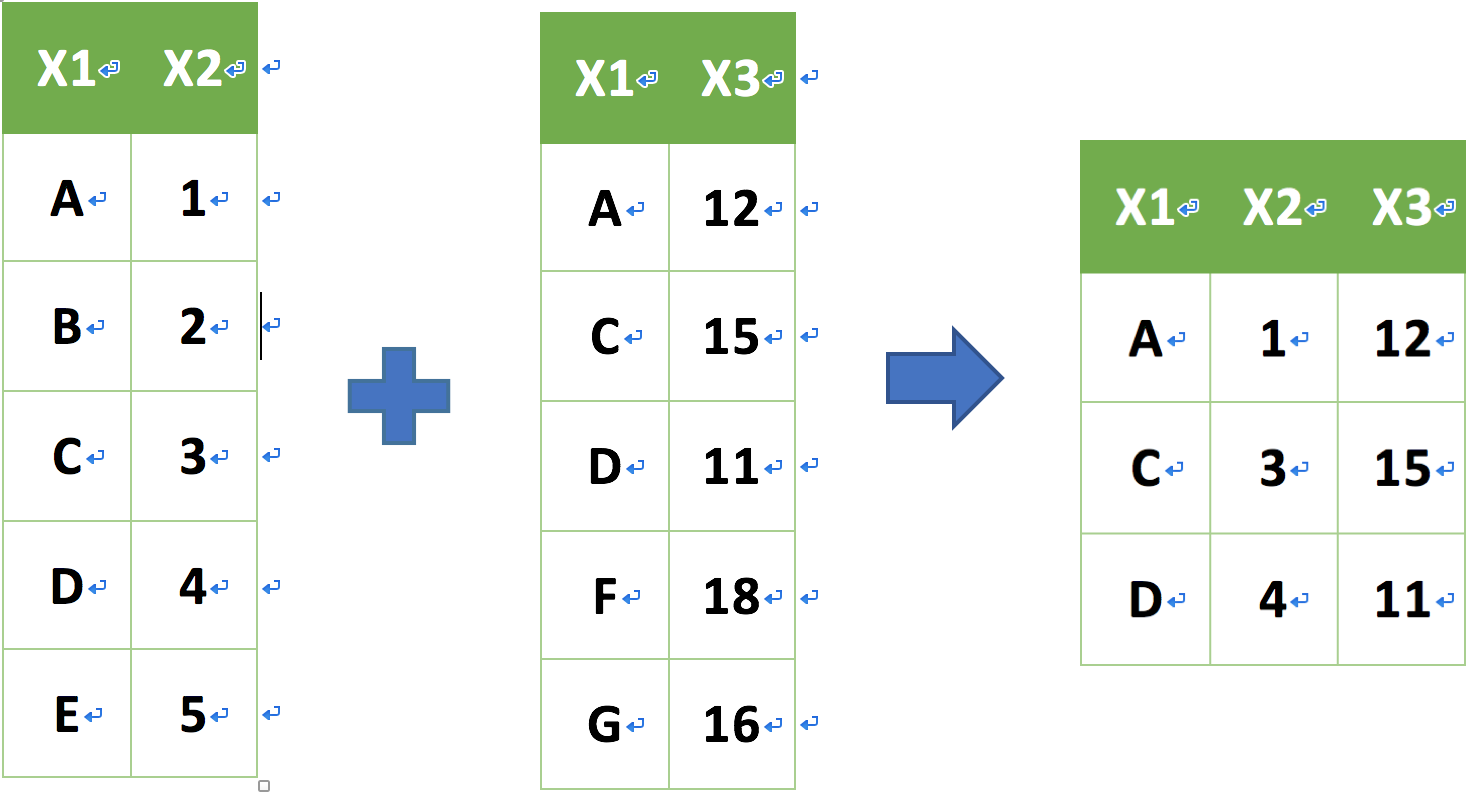
join family:inner_join
inner_join(a, b, by = "x1")
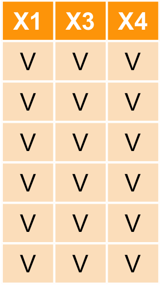
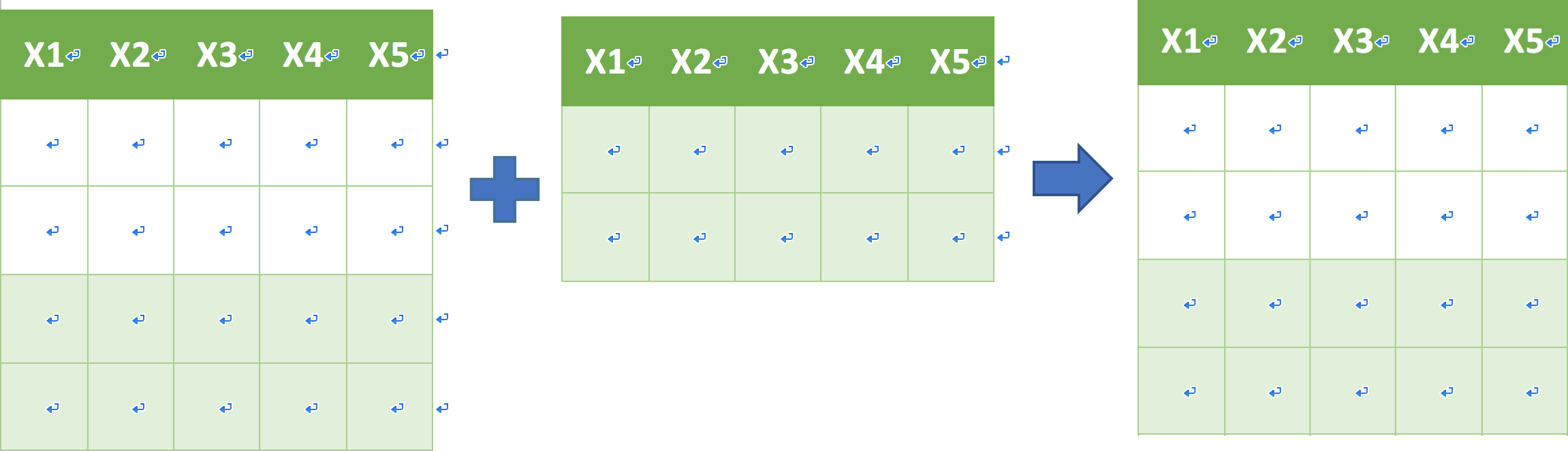
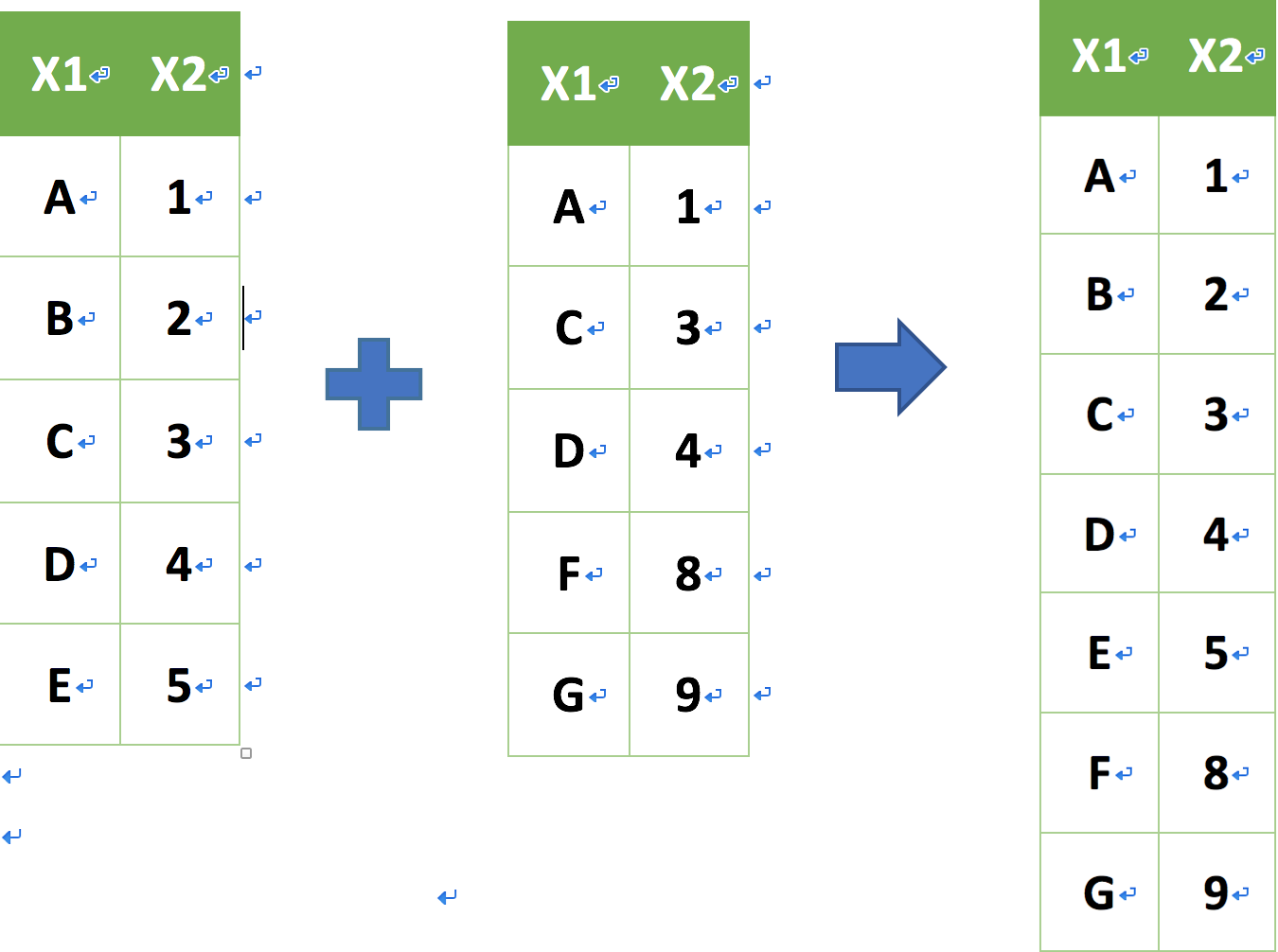
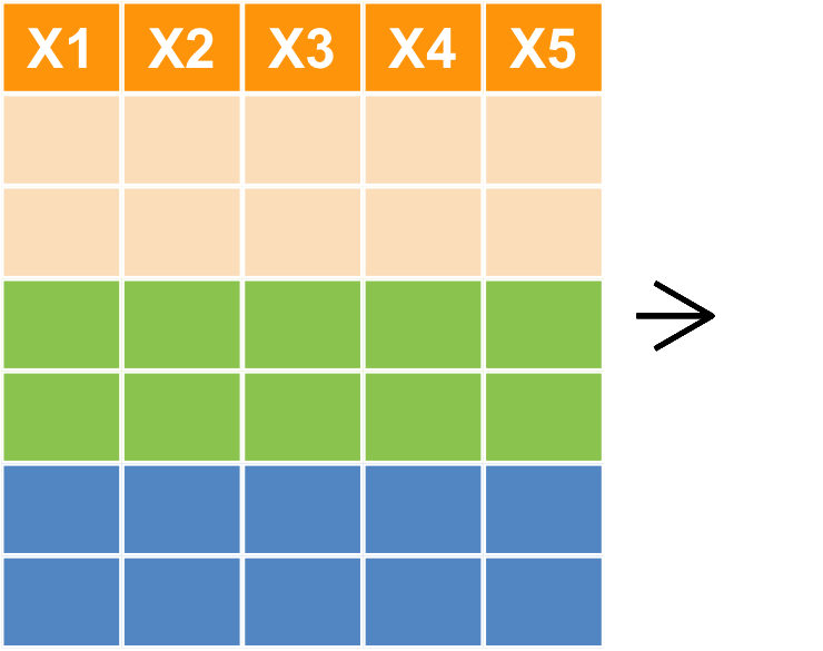
union (聯集) 資料表合併
union(a, b)
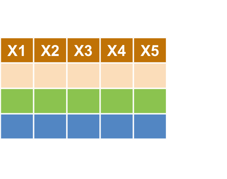
intersect (交集) 資料表合併
intersect(a, b)
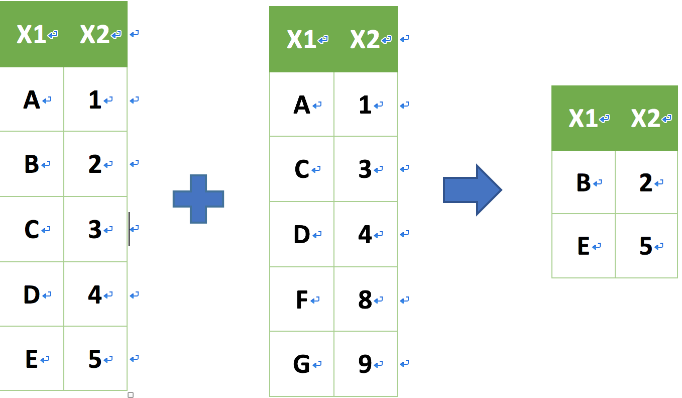
setdiff (插集) 資料表合併
setdiff(a, b)
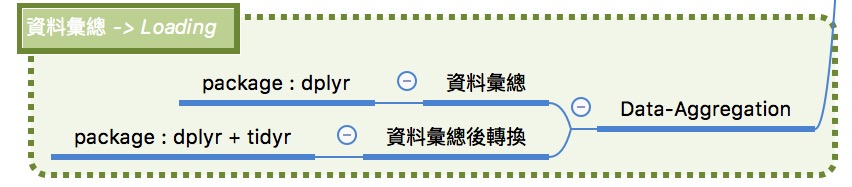
Data Aggregation : 樞紐分析
樞紐分析 group_by + summarise
樞紐分析 group_by + summarise()
- 目標:計算 各縣市 的交易筆數與平均坪價,並以高排到低。
- 利用
?dplyr::summarise查看可以擺什麼summary functionsmin(),max()n(),mean()- 更多請見 dplyr cheatsheet
樞紐分析 group_by + summarise(n())
- 利用
group_by+summarise+arrange(desc)summarise中的擺放的fun為n()=length(),表示該 group 中有幾筆資料、mean(price_unit)表示該 group 中 price_unit 平均。
transaction %>%
  group_by(city) %>%
  summarise(n = n(), mean = mean(price_unit, na.rm=T))
# A tibble: 4 x 3
    city     n   mean
  <fctr> <int>  <dbl>
1 高雄市 34460  44874
2 臺北市 24238 179345
3 臺中市 37482  50729
4 新北市 57418  94645
樞紐分析 group_by + summarise(max)
- 目標:計算 各縣市 的最高的平均坪價為多少?
transaction %>%
  group_by(city) %>%
  summarise(max_price = max(price_unit, na.rm=T))
# A tibble: 4 x 2
    city max_price
  <fctr>     <int>
1 高雄市   1902305
2 臺北市   1730511
3 臺中市   4284119
4 新北市    967864
樞紐分析小挑戰
- Tips : filter -> group_by(a,b) -> summrise() -> arrange
transaction %>%
  filter(city == '臺北市') %>%
  group_by(district, build_type) %>%
  summarise(mean = mean(price_unit, na.rm = T))
樞紐分析小挑戰之資料型態轉換
summarise 所回傳的 long-format 其實較適合我們後續畫圖(ggplot2)的資料型態,這部份各位會在下一次 EDA in R的課程中感受到!
我們利用先前學的資料型態轉換的技巧來將結果轉成方便讀比較的形式
transaction %>%
  filter(city == '臺北市') %>%
  group_by(district, build_type) %>%
  summarise(mean = mean(price_unit, na.rm = T)) %>%
  spread(build_type, mean)
Recap Today
Data ETL 的第一步:輸入資料
- 設定資料路徑:
getwd()&setwd() - 輸入不同資料型態:
- 表格式:
read.csv()&read.table() - 網頁:
readLines() - 其他軟體:
read.sas7bdat()&read.spss() - 注意編碼、路徑設定、資料內容有沒有錯誤
- 表格式:
- 輸出資料:
write.csv()
Data Manipulation:將資料操之在手。
- 字串取代/配對/長度/位置/切割:
str_
- 資料表基本操作方式:
filter挑選列select挑選欄arrange排序,mutate新增修改
- 資料表型態轉換:
gather寬轉長spread長轉寬
- 資料合併:
_join:合併資料表bind_: 合併列或欄
Data Aggregation : 樞紐分析
- 資料彙總:
group_by依照summarise彙總meam,medium,sum,max,min,n
Finally, ….
恭喜大家踏入清資料的坑!
非誠勿擾,切勿 GIGO

各位同學出作業囉 ~~
必須完成:
01-RBasic-07-Loading-Dataset02-RDataEngineer-03-JSON02-RDataEngineer-05-Data-Manipulation02-RDataEngineer-06-Join
選修:
02-RDataEngineer-01-Parsing
補充資料
繼續學習之路
- 了解自己的需求,詢問關鍵字與函數
- Taiwan R User Group,mailing list: Taiwan-useR-Group-list@meetup.com
- ptt R_Language版
- R軟體使用者論壇
- StackOverflow
- 歡迎來信 unityculturesheng@gmail.com 或其他DSP優秀教師多多交流
感謝大家!